Introduction

In this series of posts, we will cover the optimizations described in the Speeding Up Sum-Check Proving paper. To aid the explanation, we are also sharing our implementation of the algorithms in SageMath, which is available on GitHub.

The main motivation of the paper is to speed up the proving time of sumchecks for a specific case: where the values to be proven are in a small field, while the randomness is drawn from a relatively large field. For example, when proving a zkVM, we often try to prove register values that are 32-bit integers and flags that are boolean values. On the other hand, for security reasons, we often draw randomness in sumchecks from a large field, e.g. ~128-bit fields for hash-based SNARKs or ~256-bit fields for elliptic curve-based SNARKs.

This means that throughout the sumcheck protocol, the prover needs to pay for a lot of operations in the large field, which are often much slower than those in the small field.

More specifically, we can classify the arithmetic operations (we will only consider multiplications) in the sumcheck protocol into three categories:

• $\mathfrak{ss}$: small $\times$ small
• $\mathfrak{sl}$: small $\times$ large
• $\mathfrak{ll}$: large $\times$ large

And since the $\mathfrak{ll}$ multiplications are the most expensive, the paper sets out to minimize the number of these multiplications.

Preliminaries

Before diving into the optimizations, let's start with some preliminaries.

Multilinear Polynomials

Let $p: \mathbb{F}^l \to \mathbb{F}$ be a multilinear polynomial. Then, we can write it as the sum of weighted evaluations over some boolean hypercube $\{0,1\}^{l}$ using the $\tilde{eq}$ polynomial:

$$ p(x_1, x_2, \dots, x_l) = \sum\limits_{b\in\{0,1\}^{l}} \tilde{eq}((x_1, x_2, \dots, x_l), b) \cdot p(b), $$

where $x_1, x_2, \dots, x_l \in\mathbb{F}$ are variables, $p(b)$ are evaluations over the boolean hypercube, and $\tilde{eq}((x_1, x_2, \dots, x_l), b)$ are the weights.

We can remove any variable $x_i$ by iterating over the boolean values of $x_i$ and summing the results. For example, if we were to remove $x_l$, we would get the following equation:

$$ p(x_1, x_2, \dots, x_{l-1}) = \sum_{x'\in\{0,1\}^{1}} \sum\limits_{b\in\{0,1\}^{l-1}} \tilde{eq}((x_1, x_2, \dots, x_{l-1}), b) \cdot p(b,x'). $$

Similarly, we can assign any value in $\mathbb{F}$ to $x_i$. For example, we can assign $(x_1, x_2, \dots, x_{l-1}) = (r_1, r_2, \dots, r_{l-1})$ to the above equation and get the following equation:

$$ p(r_1, r_2, \dots, r_{l-1}) = \sum_{x'\in\{0,1\}^{1}} \sum\limits_{b\in\{0,1\}^{l-1}} \tilde{eq}((r_1, r_2, \dots, r_{l-1}), b) \cdot p(b,x'). $$

These two tricks are all we need in the sumcheck protocol.

Sumcheck Protocol

Throughout the sumcheck protocol, at each round $i$, we will compute a univariate polynomial for $x_i$ and evaluate it at a random value $r_i$ from the large field.

For example, in round $i=1$, we create a univariate polynomial $s_1$ as follows:

$$ s_1(X) = \sum_{x'\in\{0,1\}^{l-1}} \sum\limits_{b\in\{0,1\}^{1}} \tilde{eq}(X,b) \cdot p(b,x'). $$

Then, we evaluate $s_1$ at a random value $r_1$ from the large field and send it to the verifier, resulting in the following equation:

$$ s_1(r_1) = \sum_{x'\in\{0,1\}^{l-1}} \sum\limits_{b\in\{0,1\}^{1}} \tilde{eq}(r_1,b) \cdot p(b,x'). $$

For a general round $i$, the univariate polynomial looks like the following:

$$ s_i(X) = \sum\limits_{x'\in\{0,1\}^{l-i}} \sum\limits_{b\in\{0,1\}^{i-1}} \tilde{eq}((r_1,\dots,r_{i-1}),b) \cdot p(b,X,x'). $$

Sumcheck Over Product of Multilinear Polynomials

In this post, we will be looking at a special case where we run sumchecks on the product of $d$ multilinear polynomials $p_1, p_2, \dots, p_d$. Thus, we rewrite the equation $s_i(X)$ as:

$$ s_i(X) = \sum\limits_{x'\in\{0,1\}^{l-i}} \prod_{k=1}^d \left(\sum_{b\in\{0,1\}^{i-1}} \tilde{eq}((r_1,\dots,r_{i-1}),b) \cdot p_k(b,X,x')\right) $$

Algorithm 1: Using an evaluation table

Now we're ready to dive in!

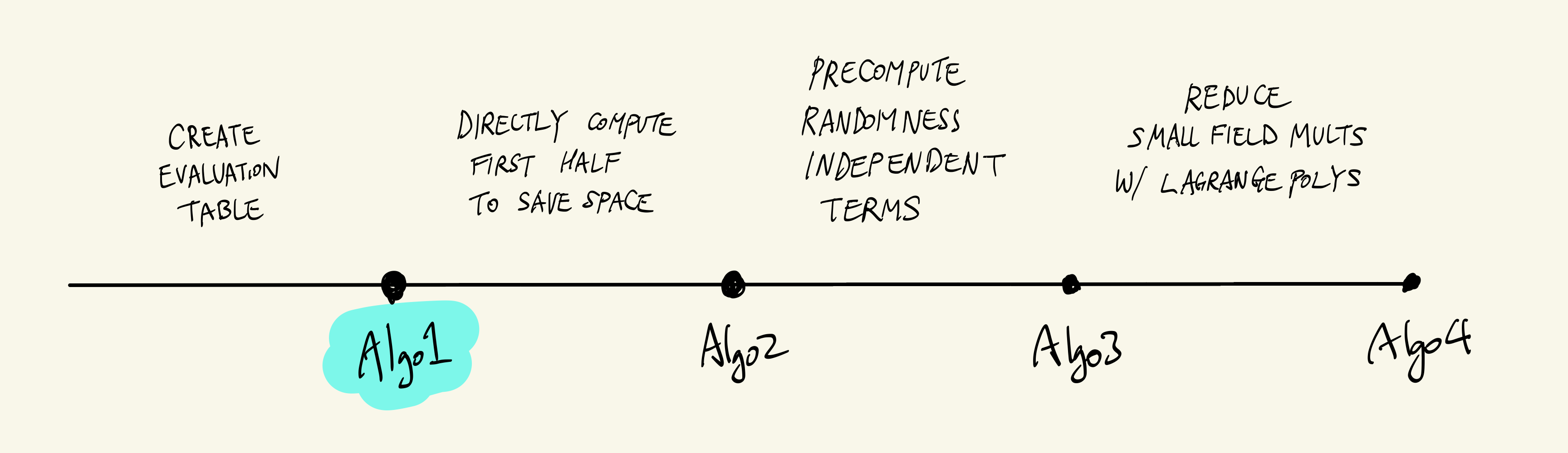
One simple way to compute $s_i(X)$ at at every round is to keep a table of all the evaluations of each $p_k(X)$ over the boolean hypercube $\{0,1\}^{l-i}$ and update it as we go through the rounds.

This involves an initial table of size $d \cdot 2^l$, with the necessary size halving at every proceeding round.

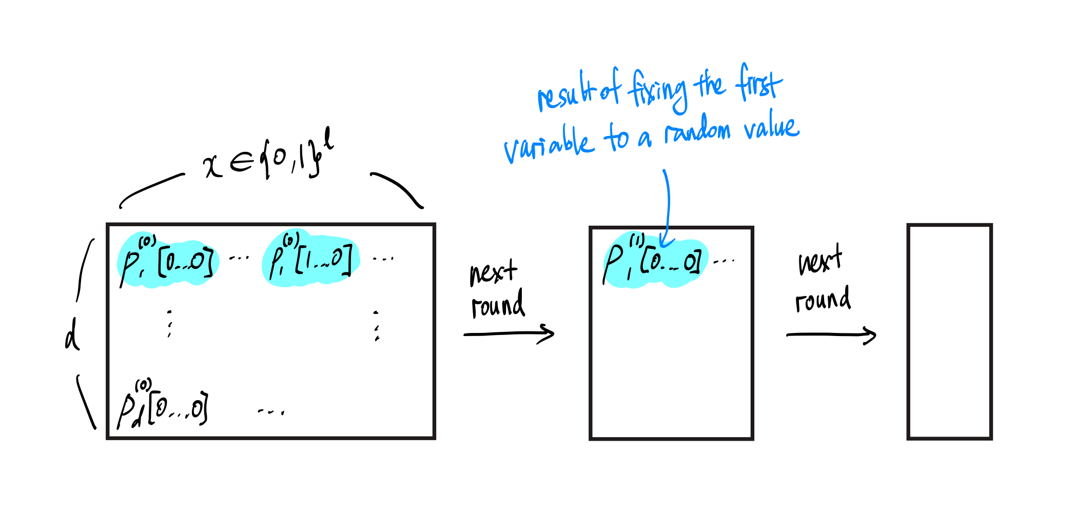
Figure 1.1: The evaluation table starting from round $i=1$.

A simple observation is that this approach is inefficient in terms of both space and time because of the initial table size and that we need to perform $\mathfrak{ll}$ multiplications beginning from the second round.

Can we do better?

Algorithm 2: Directly computing $p_k$ for each round

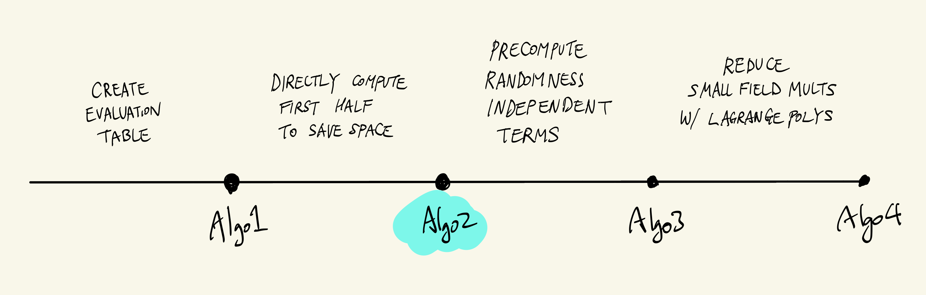
A simple solution to the space problem is to directly compute $p_k(b,X,x')$ for all $b\in\{0,1\}^{i-1}$, $x'\in\{0,1\}^{l-i}$, and $k\in[d]$ up until the size of the evaluation table becomes small enough.

For example, we can directly compute the polynomials until round $l/2$ and switch to Algorithm 1, at which point we will start with a table of size $d \cdot 2^{l/2}$ instead of $d \cdot 2^l$.

Still, we didn't solve the problem of the $\mathfrak{ll}$ multiplications beginning from the second round.

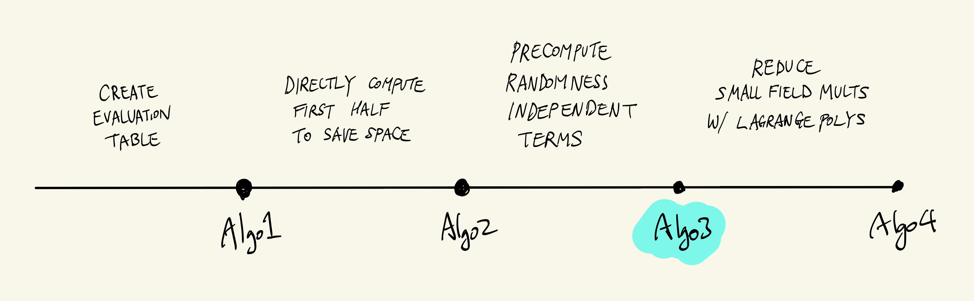
Algorithm 3: Precomputing $r$-independent terms

Separating the good from the bad

Note that once a small value is multiplied with a large value, any further arithmetic operations on the result will be a $\mathfrak{ll}$ multiplication. Thus, in order to minimize the bad ($\mathfrak{ll}$ multiplications), we will do our best to separate the good ($\mathfrak{ss}$ multiplications) from the bad by delaying multiplying the large and small values as long as possible.

Recall that the equation that the prover needs to compute is the following:

$$ s_i(X) = \sum\limits_{x'\in\{0,1\}^{l-i}} \prod_{k=1}^d \left(\sum_{b\in\{0,1\}^{i-1}} \tilde{eq}((r_1,\dots,r_{i-1}),b) \cdot p_k(b,X,x')\right). $$

You can see that this requires multiplying the $\tilde{eq}$ term (a large value) with the $p_k$ term (a small value), which will result in a large value, before iterating over all $x'$, $k$, and $b$ values.

If, however, we iterate over the $x'$, $k$, and $b$ values separately over each term and then multiply the results together, we can minimize the number of $\mathfrak{ll}$ multiplications! Plus, $p_k$ is independent of $r$, so we can precompute the values.

Let's walk through how we can do this.

First, we switch the order of the summation over $b$ with the product over $k$:

$$ \sum\limits_{x'\in\{0,1\}^{l-i}} \sum_{\boldsymbol{b}_1,..., \boldsymbol{b}_d\in\{0,1\}^{i-1}} \prod_{k=1}^d \left( \tilde{eq}((r_1,\dots,r_{i-1}),\boldsymbol{b}_k) \cdot p_k(\boldsymbol{b}_k,X,x')\right). $$

If the new summation over $\boldsymbol{b}_1,..., \boldsymbol{b}_d$ looks unfamiliar, let me remind you that the inner product now returns all $\{\boldsymbol{b}_1, \dots, \boldsymbol{b}_d\}$, so we need to iterate over all possible values of these variables.

Next, we unfold the definition of the $\tilde{eq}$ function. Note that there are two representations of $\tilde{eq}$:

$$ \begin{align} \tilde{eq}((r_1,\dots,r_{i-1}),\boldsymbol{b}_k) &= \prod_{j=1}^{i-1} (r_j \cdot \boldsymbol{b}_k[j] + (1 - r_j) \cdot (1 - \boldsymbol{b}_k[j])) \\ &= \prod_{j=1}^{i-1} (r_j^{\boldsymbol{b}_k[j]} \cdot (1 - r_j)^{1 - \boldsymbol{b}_k[j]}), \end{align} $$

and we will use the second representation.

Thus, we have the following new expression:

$$ \sum_{x'} \sum_{\boldsymbol{b}_1,..., \boldsymbol{b}_d} \prod_{k=1}^d \left(\prod_{j=1}^{i-1} \left(r_j^{\boldsymbol{b}_k[j]} \cdot (1 - r_j)^{1 - \boldsymbol{b}_k[j]}\right) \cdot p_k(\boldsymbol{b}_k,X,x')\right). $$

Let's go a bit further and exchange the product over $k$ with the product over $j$.

$$ \sum_{x'} \sum_{\boldsymbol{b}_1,..., \boldsymbol{b}_d} \left(\prod_{j=1}^{i-1} r_j^{\sum_{k=1}^{d} \boldsymbol{b}_k[j]} \cdot (1 - r_j)^{d-\sum_{k=1}^{d} \boldsymbol{b}_k[j]} \right) \cdot \left(\prod_{k=1}^d p_k(\boldsymbol{b}_k,X,x')\right). $$

Finally, let's move the sum over $x'$ inside, just before the product over $k$. We don't need to change this sum in any way since the $r$-terms do not depend on $x'$.

$$ \sum_{\boldsymbol{b}_1,..., \boldsymbol{b}_d} \left( \left( \underbrace{ \prod_{j=1}^{i-1} r_j^{\sum_{k=1}^{d} \boldsymbol{b}_k[j]} \cdot (1 - r_j)^{d-\sum_{k=1}^{d} \boldsymbol{b}_k[j]} }_{r\ \text{dependent term}} \right) \cdot \left( \underbrace{\sum_{x'}\prod_{k=1}^d p_k(\boldsymbol{b}_k,X,x')}_{r\ \text{independent term}} \right) \right). $$

As you can see, we have ended up with a multiplication of two terms, one that is dependent on the large value $r$ and another that is independent of it. Note that the number of multiplications is equal to $2^{d\cdot(i-1)}$, as we are iterating over $i-1$ bits for each of the $d$ polynomials. See below for a visual representation of a case where $d=3$ and $i=5$.

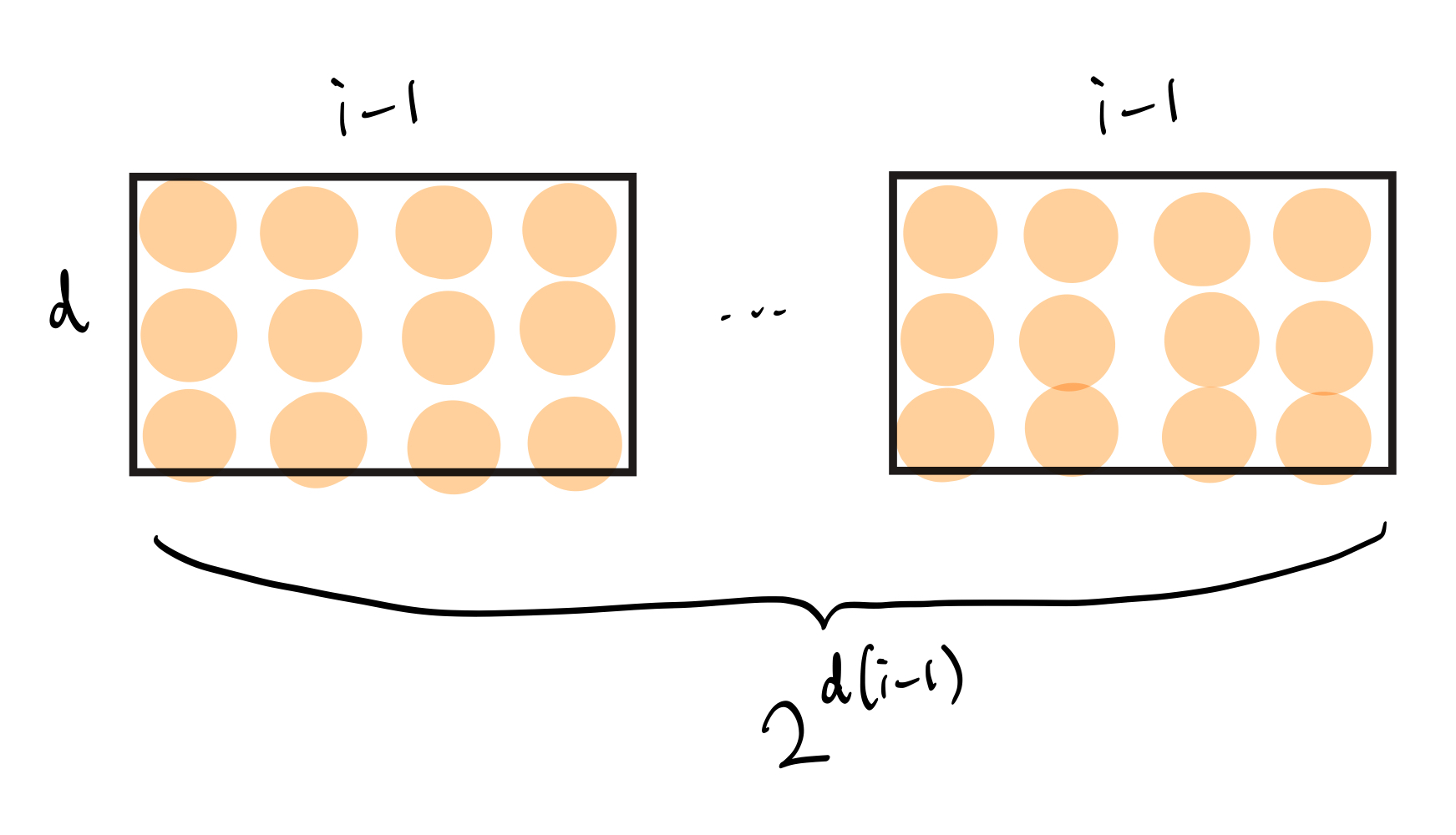
Figure 3.1: Each orange circle above represents a boolean value, and the diagram illustrates iterating over all $d \times (i-1)$ bits.

But can we make the number of multiplications smaller? Turns out we can!

Grouping $d$ bits into a single $[0,d]$ scalar value

The key observation for this optimization is that the $r$ dependent terms rely not on the individual $d\cdot (i-1)$ bits, but the sum of $d$ bits at a particular index between $1$ and $i-1$. You can see that the exponents in the following terms are summing over $d$ bits at index $j$:

$$ \prod_{j=1}^{i-1} r_j^{\sum_{k=1}^{d} \boldsymbol{b}_k[j]} \cdot (1 - r_j)^{d-\sum_{k=1}^{d} \boldsymbol{b}_k[j]}. $$

Thus, we can iterate over all possible sums of $d$ bits rather than all possible $d$ bits. Immediately, this creates an improvement from $2^d$ possible values to $d+1$ possible values (for $d$ bits, the minimum sum is $0$ and the maximum sum is $d$). Thus, the total number of iterations is reduced from $2^{d\cdot(i-1)}$ to $(d+1)^{i-1}$.

Next, we also need to change how we iterate for the term that is independent of $r$. We will iterate over the same $2^{d\cdot(i-1)}$ possible values, but in a different order.

More specifically, for each sum in $[0,d]^{i-1}$, we will iterate over all possible values of the $d$ bits that sum to the given sum. See the figure below for a visual representation of an example where $d=3$ and $i=5$.

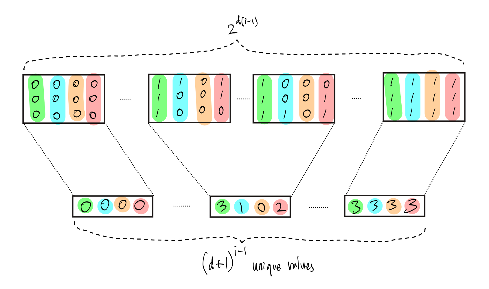
Figure 3.2: The lower rectangles represent the $(d+1)^{i-1}$ values, while the upper rectangles represent the $2^{d\cdot(i-1)}$ values, and the dotted lines show how each lower rectangle corresponds to one or more upper rectangles.

Thus, we can define a new variable $\boldsymbol{v} := (\sum_{k=1}^{d} \boldsymbol{b}_k[j])_{j\in[i-1]}$, which can be thought of one of the lower rectangles in Figure 3.2, and rewrite the equation $s_i(X)$ as follows:

$$ \sum_{\boldsymbol{v} \in [0,d]^{i-1}} \left( \underbrace{ \left( \prod_{j=1}^{i-1} r_j^{\boldsymbol{v}[j]} \cdot (1 - r_j)^{d - \boldsymbol{v}[j]} \right) }_{r\ \text{dependent term}} \cdot \underbrace{ \left( \sum_{x'} \sum_{\substack{\boldsymbol{b}_1, \ldots, \boldsymbol{b}_d \in \{0,1\}^{i-1} \\ \boldsymbol{v} = \sum_{k=1}^{d} \boldsymbol{b}_k}} \prod_{k=1}^{d} p_k(\boldsymbol{b}_k, X, x') \right) }_{r\ \text{independent term}} \right). $$

The $r$ independent term looks like a lot, but all it's doing is taking a given $\boldsymbol{v}$, or a lower rectangle in Figure 3.2, and iterating over all possible values of $\boldsymbol{b}_1,..., \boldsymbol{b}_d$ that sum up to $\boldsymbol{v}$, or all upper rectangles that are connected to the given lower rectangle.

This means that we have simply reorganized how we compute the $r$ independent term, but we have successfully reduced the amount of multiplications of the $r$ dependent and independent terms from $2^{d\cdot(i-1)}$ to $(d+1)^{i-1}$.

Precomputing the $r$ independent term, a.k.a. accumulators

Since the $r$ independent term only depends on $\boldsymbol{v}$ and $X$, we can define a new function $\mathsf{A}_i(\boldsymbol{v},X)$ as the following:

$$ \mathsf{A}_i(\boldsymbol{v},X) = \sum_{x'} \sum_{\substack{\boldsymbol{b}_1, \ldots, \boldsymbol{b}_d \in \{0,1\}^{i-1} \\ \boldsymbol{v} = \sum_{k=1}^{d} \boldsymbol{b}_k}} \prod_{k=1}^{d} p_k(\boldsymbol{b}_k, X, x'). $$

We will call this the accumulator since it accumulates all the $r$ independent values. The nice thing about this accumulator is that since it does not depend on the verifier-provided randomness $r$, we can precompute it before the sumcheck protocol starts!

Computing the $r$ dependent term incrementally

Before bringing everything together, let's see how we can simplify the $r$ dependent term:

$$ \prod_{j=1}^{i-1} r_j^{\boldsymbol{v}[j]} \cdot (1 - r_j)^{d - \boldsymbol{v}[j]} $$

Note that since $\boldsymbol{v}[j]$ for each $j\in[1, i-1]$ has $d+1$ possible values, it can be thought of as a tensor product of $i-1$ arrays of size $d+1$. For example, given $d=2$ and $i=3$, the term will be the following:

$$ [r_1^{0}\cdot(1-r_1)^2, r_1^{1}\cdot(1-r_1)^1, r_1^{2}\cdot(1-r_1)^0] \otimes [r_2^{0}\cdot(1-r_2)^2, r_2^{1}\cdot(1-r_2)^1, r_2^{2}\cdot(1-r_2)^0] $$

This indeed results in $(d+1)^{i-1}=(2+1)^{3-1} = 9$ values.

Another observation is that this tensor product can be computed incrementally, i.e. taking the tensor product of the previous round array and the new array, which has a size of $d+1$.

Thus, we can rewrite the $r$ dependent term as:

$$ \mathsf{R}_{i+1} := \mathsf{R}_i \otimes \left(r_i^k \cdot (1-r_i)^{d-k}\right)_{k=0}^{d}, $$

where the initial value is set to one: $\mathsf{R}_1 = 1$.

Bringing it all together

Now we are ready to bring everything together!

We can now rewrite the equation $s_i(X)$ as:

$$ \sum_{\boldsymbol{v} \in [0,d]^{i-1}} \mathsf{R}_i[\text{index}(\boldsymbol{v})] \cdot \mathsf{A}_i(\boldsymbol{v},X), $$

where $\text{index}(\boldsymbol{v})$ is the index of $\boldsymbol{v}$ in the array of size $(d+1)^{i-1}$.

In practice, we don't want to run this algorithm for the entire sumcheck protocol, but rather just the first few rounds and then switch to Algorithm 1. We recommend checking out Section 4.1 of the paper for more details.

Algorithm 4: The Final Algorithm

But we can still do better!

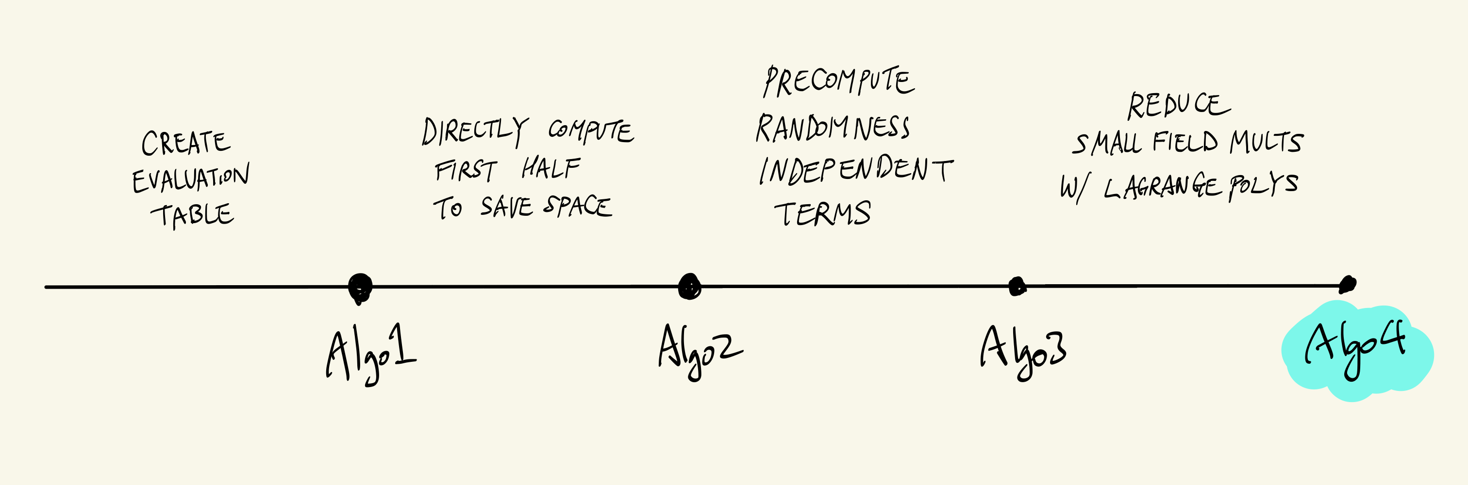
Algorithm 4 improves upon Algorithm 3 by reducing the number of $\mathfrak{ss}$ multiplications, while maintaining the number of $\mathfrak{sl}$ and $\mathfrak{ll}$ multiplications at the same level.

The main motivation is that in Algorithm 3, although there are only $(d+1)^{i-1}$ multiplications between the $r$ dependent and independent terms, we needed to iterate over all $\boldsymbol{b_1},...,\boldsymbol{b}_d\in \{0,1\}^{i-1}$, which is equivalent to $2^{d\cdot(i-1)}$ values.

So is there a way to reduce the number of iterations to $(d+1)^{i-1}$?

Simply put, we can do this by thinking of the polynomial $\prod_{k=1}^d p_k((r_1,\dots,r_{i-1}),X,x')$ as a function over $Y_1,...,Y_{i-1}$ and rewriting it as the following:

$$ F(Y_1,...,Y_{i-1}) = \prod_{k=1}^d p_k(Y_1,...,Y_{i-1},X,x'). $$

Since each $Y_1,...,Y_{i-1}$ has degree $d$, we can apply the Lagrange interpolation to each variable. Below is a step-by-step approach to the expression:

$$ \begin{align} \prod_{k=1}^d p_k(Y_1,...,Y_{i-1},X,x') &= \sum_{v_1 \in [0,d]} \mathcal{L}_{v_1}(Y_1) \cdot \prod_{k=1}^d p_k(v_1, Y_2,...,Y_{i-1}, X, x') \\ &= \sum_{v_1 \in [0,d]} \mathcal{L}_{v_1}(Y_1) \cdot \sum_{v_2 \in [0,d]} \mathcal{L}_{v_2}(Y_2) \cdot \prod_{k=1}^d p_k(v_1, v_2, Y_3,...,Y_{i-1}, X, x') \\ &= \sum_{v_1 \in [0,d]} \mathcal{L}_{v_1}(Y_1) \cdot \sum_{v_2 \in [0,d]} \mathcal{L}_{v_2}(Y_2) \cdots \sum_{v_{i-1} \in [0,d]} \mathcal{L}_{v_{i-1}}(Y_{i-1}) \cdot \prod_{k=1}^d p_k(v_1, v_2, v_3,...,v_{i-1}, X, x')\\ &= \sum_{\boldsymbol{v} \in [0,d]^{i-1}} \prod_{j=1}^{i-1} \mathcal{L}_{v_1}(Y_1) \cdot \prod_{k=1}^d p_k(\boldsymbol{v}, X, x'). \end{align} $$

where $\boldsymbol{b}_k[j]$ is the $j$-th bit of the $k$-th polynomial.

This means that we can iterate over all possible values of $Y_1,...,Y_{i-1}$ over $[0,d]^{i-1}$ and evaluate the polynomial at each vector.

Thus, we can rewrite the equation $s_i(X)$ as follows:

$$ \begin{align} s_i(X) &= \sum_{x'\in\{0,1\}^{l-i}} \sum_{\boldsymbol{v} \in [0,d]^{i-1}} \prod_{j=1}^{i-1} \mathcal{L}_{v_j}(r_j) \cdot \prod_{k=1}^d p_k(\boldsymbol{v}, X, x') \\ &= \sum_{\boldsymbol{v} \in [0,d]^{i-1}} \underbrace{ \prod_{j=1}^{i-1} \mathcal{L}_{v_j}(r_j) }_{r\ \text{dependent term}} \cdot \underbrace{ \sum_{x'\in\{0,1\}^{l-i}} \prod_{k=1}^d p_k(\boldsymbol{v}, X, x') }_{r\ \text{independent term}}, \end{align} $$

where once again, we have created an inner product of $r$ dependent and independent terms. Also, since the $\mathcal{L}_{v_j}(r_j)$ terms are independent of $x'$, we can precompute them before the sumcheck protocol starts.

Conclusion

In this post, we traced how we can optimize the sumcheck protocol for the case where the values to be proven are in a small field, while the randomness is drawn from a relatively large field.

In the next post, we will discuss how to optimize the $\tilde{eq}$ function and $\mathfrak{sl}$ multiplications in large prime fields.