Cryptography challenges @KalmarCTF 2026

KalmarCTF is one of the best-run CTFs, known for its strong organization and consistently high-quality challenges. I was honored to have the chance to guest author several cryptography challenges for the event in 2026, namely the RBG series and MissingNo.3. In this post, I will go over the two hard challenges in detail. The original challenge files and write-ups are also available on my-ctf-challenges.

While the challenges I prepared this time are not deeply centered on ZK itself, they do reflect the kinds of mistakes that commonly appear in large projects, such as unintended leakage and unsafe PRNG usage. The exploitation techniques are also relevant beyond CTF settings, as they resemble the kinds of issues that can carry real impact in security audits.

It is also worth noting that, even in the post-AI era, the two hardest challenges did not really give up their key solving ideas to LLM assistance, although LLMs could still help with parts of the coding. As a result, they ended up with only 2 and 1 solves, respectively.

MissingNo.3

print(f'Sage version = {version()}')

set_random_seed(input("seed: "))

F = GF(0xdead1337cec2a21ad8d01f0ddabce77f57568d649495236d18df76b5037444b1)
A = random_matrix(F, 52)[:,:-3]

# github.com/AustICCQuals/Challenges2025/blob/main/crypto/missingno/publish/Ab.sobj
if A == load("Ab")[0]:
    print("kalmar{...}")

The original challenge was designed as a fun problem centered around extension fields and the LLL algorithm. However, while investigating it further, I found that SageMath's PRNG implementation allowed the internal state to be recovered completely from the random_matrix output used in the challenge.

The Backend Algorithm

The base field order given in the challenge,

0xdead1337cec2a21ad8d01f0ddabce77f57568d649495236d18df76b5037444b1,

factors as 6821063305943^6. Internally, SageMath generates random matrices over this field by filling each entry with R.random_element(...):

...
if density >= 1:
    for i from 0 <= i < self._nrows:
        for j from 0 <= j < self._ncols:
            self.set_unsafe(i, j, R.random_element(*args, **kwds))
...

For an extension field, random_element() constructs an element coefficient by coefficient over the base ring:

...
rand = current_randstate().python_random().random
R = self.base_ring()
v = self(0)
prob = float(prob)
for i in range(self.rank()):
    if rand() <= prob:
        # prob is equal to 1 in default, so this branch is always ran.
        v[i] = R.random_element(*args, **kwds)
return v

At the base field level, this eventually becomes:

...
if self.degree() == 1:
    return self(randrange(self.order()))

Therefore, random matrix generation over this field can be viewed, in essence, as repeatedly executing the following pattern, with the randrange outputs known to us:

random()
randrange(6821063305943)

Mersenne Twister

SageMath internally uses the Mersenne Twister as its default fast PRNG. Because it is entirely linear, it is unsuitable for security-sensitive use. By default, it produces 32-bit unsigned integers, and various higher-level random functions are built on top of this primitive. From this point on, I will refer to it as getrandbits32.

The random function consumes two calls to getrandbits32 and combines them into a C double, while randrange is implemented using rejection sampling.

Since $2^{42} < 6821063305943 < 2^{43}$, randrange(6821063305943) first generates a 43-bit candidate using two calls to getrandbits32. If the resulting value is at least 6821063305943, it is rejected and a new 43-bit candidate is generated. This process repeats until a value smaller than 6821063305943 is obtained, which is exactly how rejection sampling works.

While the Mersenne Twister is linear over $\mathbb{F}_2$ at the bit level, meaning that an attacker can easily recover its full internal state once 19937 independent output bits are known, rejection sampling obscures the exact alignment between observed outputs. In other words, the gaps between outputs become unknown, so the standard approach no longer applies directly and a different method is required.

A standard trick for dealing with rejection sampling is to exploit structural relations between specific output indices that arise from the PRNG's internal recurrence.

def check(v0, v396):
    if None in [v0, v396]:
        return None
    v0, v396 = [untemper(v % 2**32) for v in [v0, v396]]

    cand = []

    for m in range(2):
        y = (m * 0x80000000) + (v0 & 0x7fffffff)
        v = v396 ^ (y >> 1)
        if y & 1:
            v ^= 0x9908b0df
        v623 = v

        cand.append(temper(v623))

    return cand

l = 50000
a = [getrandbits(32) for _ in range(l)]

for i in trange(l - 2000):
    v0, v396, v623 = a[i], a[i + 396], a[i + 623]
    assert v623 in check(v0, v396)

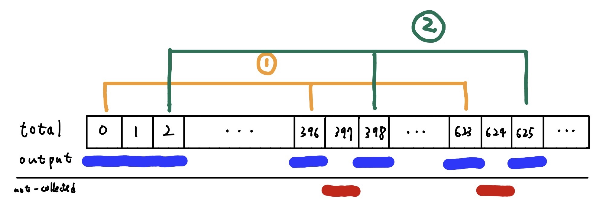
In particular, every triple of 32-bit outputs at indices [i, i+396, i+623] satisfies a specific relation. Because one extra bit is needed to determine the relation completely, each pair (v0, v396) yields two possible candidates for v623. As a result, a uniformly random triple satisfies this constraint with probability only $\frac{1}{2^{31}}$.

This idea can be applied to rejection sampling based challenges as follows. One tries many triples of observed outputs and checks whether they satisfy the corresponding consistency relation. Whenever a triple passes the test, it strongly suggests that those three outputs are separated by the exact internal offsets required by the Mersenne Twister recurrence. By collecting enough such relations and combining them with external tools such as an SMT solver, one can recover the missing index alignment and eventually reconstruct the full Mersenne Twister state.

However, this approach does not apply directly to the challenge. Each random call consumes two getrandbits32 outputs, and randrange(6821063305943) also consumes two. In the latter case, the first 32-bit word is reflected in the output in full, whereas the second contributes only its lower $43 - 32 = 11$ bits. As a result, fully observed 32-bit values appear only at even offsets.

The difficulty is that the Mersenne Twister relation at offsets [0, 396, 623] necessarily involves both even and odd positions. Therefore, at least one of the three values involved in such a relation must come from one of these truncated 11-bit observations rather than a full 32-bit word. This raises the false-positive probability significantly: instead of being $\frac{1}{2^{31}}$, it becomes $\frac{1}{2^{10}}$. This is extremely high for a system that requires many relations as possible.

Finding even offset 3-relations

This is the key idea on solving this challenge. with connecting multiple 3-relation above, we can achieve an another 3-relation with all same parity.

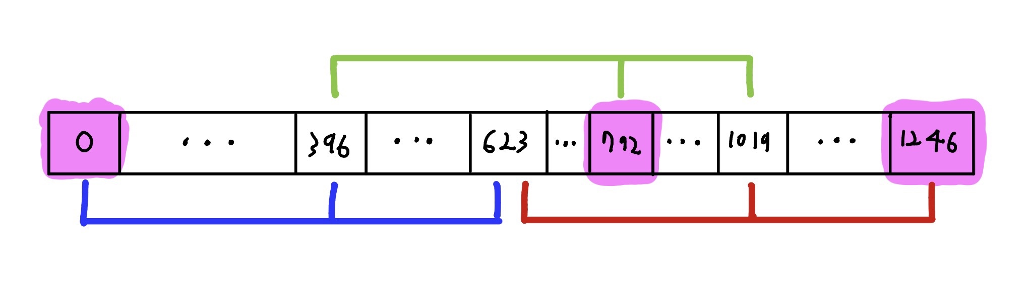
By combining three such 3-relations at different offsets, one finds that the indices [0, 792, 1246] are all even, while the middle indices [396, 623, 1019] each appear in two relations and are therefore constrained twice. Experimentally, part of the freedom of intermediate terms cancels out. As a result, the combined relation retains information only about the target indices [0, 792, 1246], which are exactly the positions we need. In particular, the value v396_dummy in the code below can be replaced with any other 32 bit integer, and the relation still holds.

def check2(v0, v792):
    if None in [v0, v792]:
        return None
    v0, v792 = [untemper(v % 2**32) for v in [v0, v792]]

    v396_dummy = 0

    cand = []

    for m1, m2, m3 in itertools.product(range(2), repeat=3):

        y = (m1 * 0x80000000) + (v0 & 0x7fffffff)
        v = v396_dummy ^ (y >> 1)
        if y & 1:
            v ^= 0x9908b0df
        v623 = v

        y = (m2 * 0x80000000) + (v396_dummy & 0x7fffffff)
        v = v792 ^ (y >> 1)
        if y & 1:
            v ^= 0x9908b0df
        v1019 = v

        y = (m3 * 0x80000000) + (v623 & 0x7fffffff)
        v = v1019 ^ (y >> 1)
        if y & 1:
            v ^= 0x9908b0df
        v1246 = v

        cand.append(temper(v1246))

    return cand

l = 50000
a = [getrandbits(32) for _ in range(l)]

for i in trange(l - 1246):
    v0, v792, v1246 = a[i], a[i + 396 * 2], a[i + 623 * 2]
    assert v1246 in check2(v0, v792)

With this, we can find relations with three 32 bit integers, with false positive probability of $\frac{1}{2^{29}}$ which is small enough.

Misc.

For my own solve, I also explored a few approaches other than the 3-relation for [0, 792, 1246]. One useful source of additional information was to check whether two consecutive [0, 396, 623] relations both held and then mark that case as valid. Since this test simultaneously involves two samples containing only 11-bit information, its false-positive probability is much smaller than $\frac{1}{2^{10}}$, making it practical to use.

Even after collecting many such relations, the system is still not constrained enough to recover the state directly. Instead, an SMT solver can be used to merge connected clusters of offsets while testing multiple possible gap assignments. For each candidate merge, one can either rely on the SMT solver itself or check, from a linear-algebraic perspective, whether the recovered bits are consistent with a valid MT19937 output sequence. Checking both is the most helpful. Repeating this process gradually merges the clusters, until the accumulated constraints reach full rank 19937 and the entire state can be recovered.

The final steps require a little bit more of source reading of Mersenne Twister seeding algorithm, and GMP's seeding algorithm, which isn't too hard but include some fun field arithmatics.

RBG+++

from Crypto.Util.number import *

PBITS, NDAT = 137, 137

with open("flag.txt", "rb") as f:
    m = int.from_bytes(f.read())

N = getPrime(PBITS) * getPrime(PBITS)
e = getRandomRange(731, N)
print(f"{N = }")

lcg = lambda s: (s * 3 + 1337) % N

for i in range(NDAT):
    print(pow(m, e:=lcg(e), N) + pow(m, e:=lcg(e), N))

    # Internal audit
    e = getRandomRange(731, N)
    print(f"[DEBUG] {e = }")

This challenge is relatively more brainstorming than audit style library reading challenges and thus the challenge file is very simple without any imports.

The previous challenges in the RBG series revolved around arithmetic over RSA-style composite moduli and polynomial arithmatics over them, in the spirit of Franklin-Reiter type challenges. This one may look similar at first glance, but a small twist pushes it in a more creative direction.

Overview

The modulus $N$ is an RSA-style composite, but its prime factors are only 137 bits long, so factoring it is trivial. Let $N = pq$.

A linear congruential generator (LCG) is defined by

Finally, we are given 136 values of the form

Now observe that for a uniformly random exponent $e$, we have

for some $k \in {0,1,2}$, and each case occurs with probability roughly $\frac{1}{3}$.

Suppose we collect all instances with $k=0$. Then for each such sample, we have

Since $p$ is now a known prime, the natural question is: can we recover $m$ from these equations?

For univariate polynomials over a finite field, finding roots is usually straightforward when the degree is small: one can factor the polynomial directly, or even apply a polynomial GCD-style approach when given two or more related instances. In this case, however, the equations are extremely sparse polynomials with enormous degree, so treating them as ordinary univariate polynomials is infeasible.

Idea of an easier challenge

What if we were given values of the form $m^{e_i}+m$, instead of $m^{e_i}+m^{3e_i+1337}$?

Then each sample becomes

so every huge power $m^{e_i}$ can be replaced by a linear polynomial in $m$.

Now use Fermat's little theorem, $m^{p-1}\equiv 1 \pmod p,$ so exponents can be reduced modulo $p-1$. More generally, if we can find a short relation

with small integer coefficients $a_i$, then

Substituting $m^{e_i}\equiv c_i-m$ turns the left-hand side into a rational expression in $m$, and after clearing denominators we obtain a low-degree polynomial equation in $m$.

So the task reduces to finding a short modular relation among the exponents, which is exactly the kind of structure LLL can help uncover.

Realistically, say there are only 10 samples we can use. Since $p$ is a 137-bit prime, we are looking for a relation

in a space of size about $2^{137}$. Heuristically, if we allow coefficients $|a_i|\le B$ and also aim for a small residue $|r|\le B$, then the number of candidate relations is about $(2B+1)^{10}(2B+1)\approx (2B)^{11}$. Matching this against $2^{137}$ gives

so

This places the coefficients in the low-thousands range. After substituting $m^{e_i}\equiv c_i-m$, the resulting polynomial degree is governed by the total coefficient size, so one naturally expects a degree around $10^4$, which is comfortably within the range where roots can be found.

The original challenge

Now how can we apply this idea using the LLL algorithm to the original challenge?

Define $x=m^{-1337}$. Then each sample in that branch can be rewritten as

If we let $A_i=m^{e_i}$, this becomes the cubic relation

At this point, the problem has been transformed into a system of low-degree algebraic equations in the variables $A_i$ and $x$. The remaining issue is how to connect the different $A_i$'s. Since we are working modulo a prime $p$, exponents live modulo $p-1$. This means we may view each $A_i$ as a power of $x$.

With the equal idea from the easier challenge, we can find short coefficients and final result using LLL algorithm again. We search for small integers $s_i$ and a small residue $s$ such that

Equivalently, $\prod_i A_i^{s_i}=x^s$. So LLL gives us a way to express a product of the unknown $A_i$'s as a comparatively small power of $x$.

Once such a relation is found, we combine it with the cubic equations

and eliminate the variables $A_i$ one by one using resultants. After all $A_i$ are removed, what remains is a univariate polynomial in $x$ over $\mathbb{F}_p$. Its roots include the correct value of $x$, so we can solve for $x$ modulo $p$.

Once $x$ is known, recovering $m$ is straightforward from $x=m^{-1337}$, and we solve the challenge!

Misc.

A few notes that are worth mentioning.

• The implementation is much more involved than the algebraic sketch above.
• In my solve, the final univariate polynomial had degree around $10$M to $20$M, which is still workable but large enough that one should avoid expensive tricks like computing $\gcd\bigl(x^p-x \bmod f(x),f(x)\bigr)$ via a full modular exponentiation inside the polynomial ring.
• My final solve took about 17 core-hours, which is not small but not overly long for a hard ctf challenge.

Thankfully the only solver, Sceleri, wrote an excellent write-up on his blog, so I highly recommend checking it out for a solver's perspective as well.