Kocher's Timing Attack: A Journey from Theory to Practice

In 1996, Paul Kocher published a seminal paper demonstrating that the execution time of cryptographic operations could leak information about secret keys. This wasn't a mathematical weakness in the abstract cryptographic algorithms, but rather a side-channel attack that exploited efficient implementations. This work opened an entire field of side-channel cryptanalysis, showing that physical implementations leak information in unexpected ways.

This tutorial explores timing attacks through three progressive implementations, each revealing different aspects of the challenge. We first start with a simple instruction cost model to illustrate the core dynamics of the attack. We then move on to actual timing measurements on more realistic implementations and show the challenges presented by modern processors and operating systems. Finally, we show some engineering techniques to recover the key signal from noisy measurements. This progression illustrates both the theoretical foundations and practical engineering challenges of side-channel cryptanalysis.

Preview and Download the Interactive Notebook to follow along with working code, or simply read the post standalone.

The Vulnerable Algorithm

At the heart of both RSA encryption and Diffie-Hellman key exchange is modular exponentiation: computing $m^k \bmod n$. The naive approach of multiplying the base $k$ times would require millions of operations for typical cryptographic keys. Instead, implementations often use the efficient square-and-multiply algorithm that reduces this to roughly $\log k$ operations.

The algorithm processes the exponent bit by bit. For each bit, it always squares the current base. But here's the crucial detail: when the current bit is 1, it performs an additional multiplication. This conditional operation creates the vulnerability:

def fast_exp(base, exponent, modulus):
    result = 1
    base = base % modulus
    while exponent > 0:
        if exponent & 1:            # THE LEAK: extra work when secret bit = 1
            result = (result * base) % modulus
        base = (base * base) % modulus
        exponent >>= 1
    return result

When a secret key bit is 1, the algorithm performs an extra multiplication. When the bit is 0, it skips that step. This creates a measurable timing difference between the two cases. Kocher's breakthrough was realizing that statistical analysis of many such measurements could recover the entire secret key, bit by bit.

Part 1: Clean Signal, Clean Results

Note that when computing multiplication of two numbers $a \cdot b$ modulo $n$, the result of a multiplication may be smaller or bigger than $n$, which in turns implies that $a \cdot b$ may need reduction modulo or not. This in turn implies that not all messages $m$ will take the same amount of time when computing $m^k \bmod n$ for the same key $k$. This variability of timing for multiple messages and a fixed key will be crucial for our exploitation strategy.

To illustrate the attack, instead of wrestling with noisy wall-clock measurements, we use a simple cost model: every modular multiplication costs one multiply plus however many "trial subtractions" are needed to reduce the result. This toy model captures the essential timing variation without system interference. Note that in practice more efficient multiplication modulo algorithms are used, but as we will see next, they also induce a similarly distributed instruction variability.

def mul_mod_with_cost(a, b, n):
    """Multiply with realistic cost modeling via trial subtraction"""
    x = a * b
    k = x // n
    x = x - k * n
    return x, 1 + int(k)

def fast_exp_with_cost(base, exponent, modulus):
    """LSB-first square-and-multiply with cost counting"""
    result = 1
    base = base % modulus
    total_cost = 0

    while exponent > 0:
        if exponent & 1:  # vulnerable conditional
            result, mul_cost = mul_mod_with_cost(result, base, modulus)
            total_cost += mul_cost

        base, square_cost = mul_mod_with_cost(base, base, modulus)
        total_cost += square_cost

        exponent >>= 1

    return result, total_cost

As we can see, the number of instructions (costs, or time) follows a normal distribution as many small random costs add up. This provides an ideal statistical foundation for Kocher's variance distinguisher.

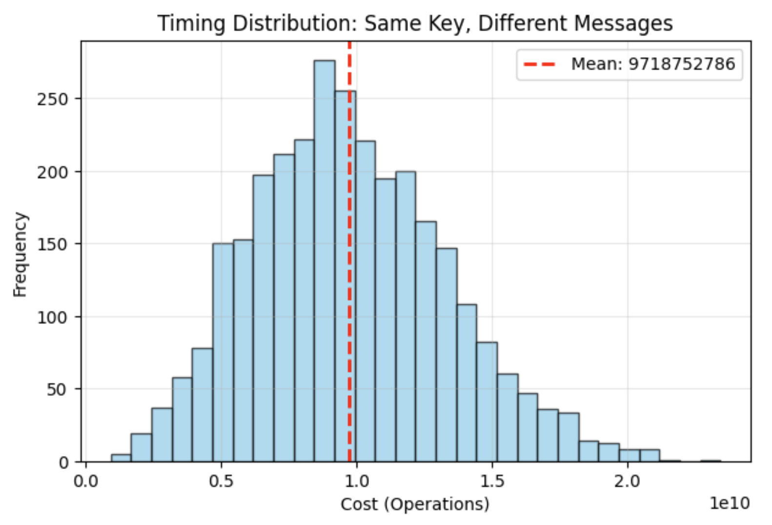Figure 1: Clean normal distributions enable reliable statistical analysis.

The approximately normal distribution of timing costs can be explained by the central limit theorem: modular reductions introduce many small, message-dependent variations that behave like independent noise terms. Summed across rounds, these variations converge to a bell-shaped distribution. This motivates treating the timing of each round as approximately independent, which is exactly the assumption Kocher’s variance distinguisher relies on to decompose total variance into separate contributions.

We can validate this independence assumption empirically. When we measure the correlation between the timing of early rounds (say, the first 4 rounds) and later rounds across many messages, we consistently observe coefficients below 0.1. Such values indicate very weak dependence, which supports treating the rounds as approximately independent for the purposes of Kocher’s variance analysis.

Kocher's Variance Distinguisher Theory

The key insight is that if round timings are independent, variance decomposes additively. For any exponentiation with total cost $T_m$, we can write:

where $\text{prefix}_m^{(i)}$ covers the first $i$ rounds and $\text{suffix}_m^{(i)}$ covers the remainder.

When we subtract the correct hypothesis for the prefix:

When we subtract an incorrect hypothesis, we get an additional error term:

Since the error $\Delta_m^{(i)}$ is independently distributed across messages:

Therefore: $\text{Var}[\text{correct}] < \text{Var}[\text{wrong}]$

The distinguisher simply compares variances: the hypothesis that produces lower variance when subtracted from the baseline measurements is more likely to be correct. This mathematical foundation enables bit-by-bit key recovery through statistical analysis.

🔓 FULL LSB KEY RECOVERY ATTACK
==================================================
Target key: 55 = 0b110111
Assuming bit 0 (LSB) = 1 for RSA exponents
Recovering bits 1 to 5 (LSB+1 to MSB)...

Attacking bit 1 (LSB+1)
  H0 error variance: 1.10e+19
  H1 error variance: 9.70e+18
  Winner: H1
  Predicted: 1 ✅

Attacking bit 2 (LSB+2)
  H0 error variance: 7.61e+18
  H1 error variance: 7.24e+18
  Winner: H1
  Predicted: 1 ✅

Attacking bit 3 (LSB+3)
  H0 error variance: 5.96e+18
  H1 error variance: 6.14e+18
  Winner: H0
  Predicted: 0 ✅

[... continued ...]

🎯 FINAL RECOVERY ANALYSIS
Target key:     55 = 0b110111
Recovered key:  55 = 0b110111
Accuracy: 6/6 = 100.0%

For this simple cost model we obtain a complete recovery with all bits correctly identified. Can we reproduce these results by measuring wall-clock time instead of using the toy model?

Part 2: The Challenge of Real Systems

Modern computers introduce multiple sources of timing variability. The operating system interrupts processes to handle other tasks. The CPU adjusts its clock speed based on temperature and workload. Memory caches create variable delays. Moreover, Python's garbage collector introduces timing spikes. This means the same variance distinguisher that worked reliably in Part 1 is not guaranteed to work effectively.

First, let us have a look at the distribution of time measurements for the same key as we did in Part 1. We want to check if the normal distribution still holds, which was the hint we used to deduce that the time per round was random and independent from round to round.

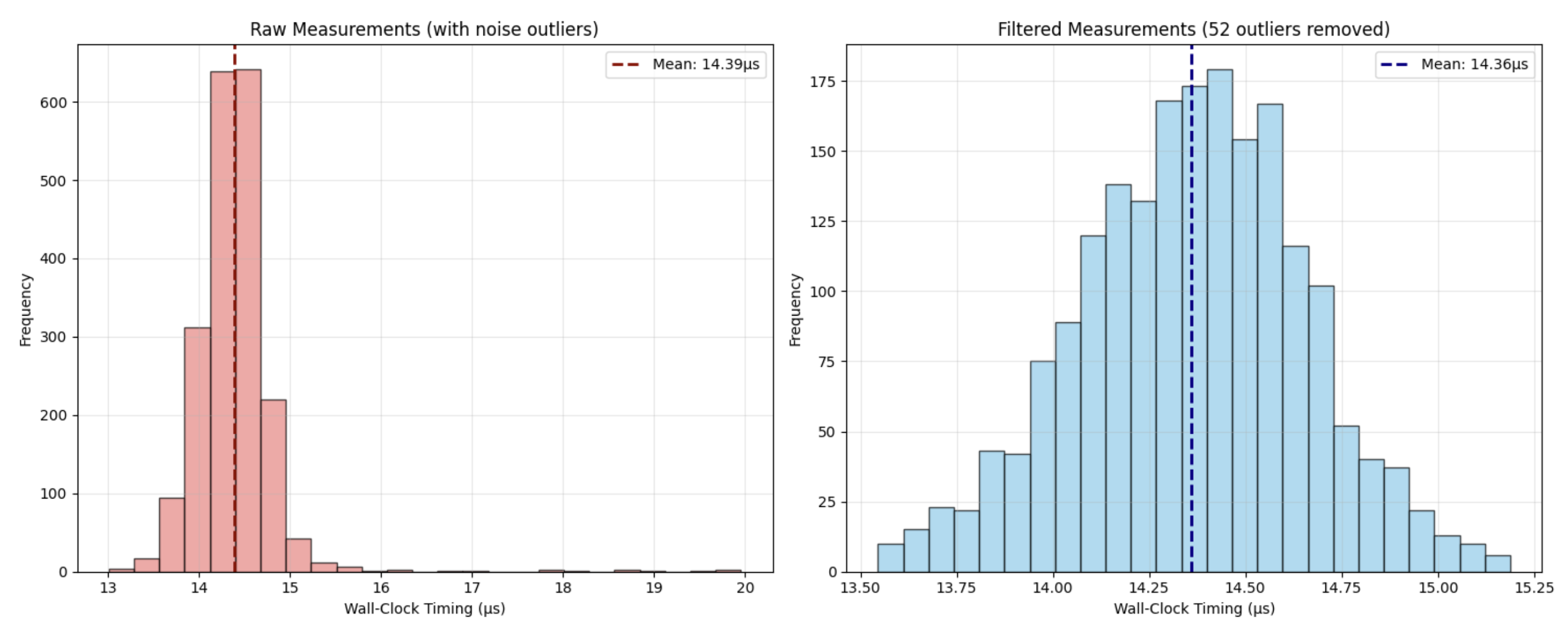Figure 2: Distribution of wall clock measurements is also normal after removing outliers

As we can see a similar distribution seems to be there after removing outliers, suggesting the feasibility of our attack for timing measurements. Let us try to directly reproduce our attack, using a 100x amplification of the time measurement to avoid noise from harming the exploit.

Part 2 Demonstration
==================================================
Target key: 53 (0b110101)
Modulus: 512-bit prime
Timing source: Wall-clock (realistic noise)
Algorithm: LSB-first with assumed first bit = 1

Reality Check - Naive Wall-Clock Timing Attack
============================================================
Target key: 53 (binary: 0b110101)
Messages: 3000
Amplification: 100 iterations per measurement

Step 1: Generating random messages...
Generated 3000 random messages

Step 2: Collecting baseline measurements (full exponentiation)...
Warning: This uses wall-clock timing - expect noise!
Baseline complete. Mean: 11.491μs, Std: 0.320μs
Coefficient of variation: 2.8% (high = noisy!)

Step 3: Attempting to recover 5 bits...
Warning: With high noise, variance distinguisher becomes unreliable

🔑 Exponent Assumption:
  Bit 0 (LSB): 1 (assumed known and odd)
  Starting attack from bit 1 (second LSB)...

--- Attempting bit 1 (LSB+1) ---
Testing H0: 32769 = 0b1000000000000001 (bit 1 = 0)
Testing H1: 32771 = 0b1000000000000011 (bit 1 = 1)
Actual bit value: 0
Measuring noisy wall-clock timings...
Prediction means: H0=2.435μs, H1=3.773μs
Error variances: H0=0.11, H1=0.11
Decision: bit = 1
Result: ✗ WRONG

--- Attempting bit 2 (LSB+2) ---
Testing H0: 32771 = 0b1000000000000011 (bit 2 = 0)
Testing H1: 32775 = 0b1000000000000111 (bit 2 = 1)
Actual bit value: 1
Measuring noisy wall-clock timings...
Prediction means: H0=4.994μs, H1=6.366μs
Error variances: H0=0.10, H1=0.09
Decision: bit = 1
Result: ✓ CORRECT

--- Attempting bit 3 (LSB+3) ---
Testing H0: 32775 = 0b1000000000000111 (bit 3 = 0)
Testing H1: 32783 = 0b1000000000001111 (bit 3 = 1)
Actual bit value: 0
Measuring noisy wall-clock timings...
Prediction means: H0=7.638μs, H1=9.045μs
Error variances: H0=0.09, H1=0.10
Decision: bit = 0
Result: ✓ CORRECT

--- Attempting bit 4 (LSB+4) ---
Testing H0: 32775 = 0b1000000000000111 (bit 4 = 0)
Testing H1: 32791 = 0b1000000000010111 (bit 4 = 1)
Actual bit value: 1
Measuring noisy wall-clock timings...
Prediction means: H0=8.803μs, H1=10.185μs
Error variances: H0=0.08, H1=0.09
Decision: bit = 0
Result: ✗ WRONG

--- Attempting bit 5 (LSB+5) ---
Testing H0: 32775 = 0b1000000000000111 (bit 5 = 0)
Testing H1: 32807 = 0b1000000000100111 (bit 5 = 1)
Actual bit value: 1
Measuring noisy wall-clock timings...
Prediction means: H0=10.007μs, H1=11.400μs
Error variances: H0=0.07, H1=0.08
Decision: bit = 0
Result: ✗ WRONG

============================================================
FINAL RESULTS
============================================================
Target key:     53 (0b110101)
Recovered key:  7 (0b111)
Accuracy: 3/6 bits correct (50.0%) (includes assumed LSB)

As we can see the attack achieves only 50% accuracy, which is equivalent to random guessing. Notice how the error variances are nearly identical across all attempts (0.11 vs 0.11, 0.10 vs 0.09, 0.09 vs 0.10), making the distinguisher unable to reliably tell which hypothesis is correct. Even with 3000 messages and 100x amplification, the signal remains buried in noise.

This failure illustrates an important lesson: theoretical vulnerabilities and practical exploitation can be quite different. The microsecond timing differences that appeared clear in Part 1 are overwhelmed by system noise measured in the same microseconds. Real-world timing attacks require more sophisticated measurement techniques than simply timing algorithm execution.

Part 3: Engineering Solutions

Can we do better than Part 2? The answer lies in systematic engineering that addresses each source of variability. Python's garbage collector introducing timing spikes? Disable it during timing loops. CPU caches and branch predictors causing startup effects? Add warm-up runs. Systematic drift between measurements? Alternate the order you test hypotheses. Outlier measurements from context switches? Filter them out using robust statistics.

Here are some of the techniques we used to improve the attack:

import numpy as np
import random
import time
import gc

def iqr_filter(data, factor=1):
    if len(data) < 4:
        return data
    data = np.array(data)
    q1 = np.percentile(data, 25)
    q3 = np.percentile(data, 75)
    iqr = q3 - q1
    if iqr == 0:
        return data.tolist()
    lower = q1 - factor * iqr
    upper = q3 + factor * iqr
    filtered = data[(data >= lower) & (data <= upper)]
    if len(filtered) < len(data) * 0.5:
        lower = q1 - 3.0 * iqr
        upper = q3 + 3.0 * iqr
        filtered = data[(data >= lower) & (data <= upper)]
    return filtered.tolist()


def measure_timing_simple(operation, amplification=5000, num_runs=10):
    gc_was_enabled = gc.isenabled()
    gc.disable()
    try:
        times = []
        for _ in range(10):
            operation()
        for run in range(num_runs):
            if run > 0:
                time.sleep(0.001)
            start = time.perf_counter()
            for _ in range(amplification):
                operation()
            elapsed = time.perf_counter() - start
            times.append((elapsed * 1e6) / amplification)
        times_clean = iqr_filter(times)
        return np.median(times_clean)
    finally:
        if gc_was_enabled:
            gc.enable()

Let us now test our techniques against a similar target to Part 2. We will still use a random 512 modulus, but this time instead of 3000 messages we will use only 1200. We will use a higher amplification at 1000x which we will repeat 3 times to further smooth out noise. Last, we will bias the measurements to the 80% of messages that have the bigger delta between hypothesis to make the error more visible for the distinguisher. To keep the experiment relatively fast to run in our Python notebook we will assume the first 7 bits of the key are already known, and we will focus on recovering the next 3 bits.

Part 3 Demonstration: Robust Timing Attack
============================================================
Target key: 2475 (0b100110101011)
Key length: 12 bits
Modulus: 512-bit prime modulus

🔧 Engineering Solutions:
• Drift-resistant measurements with order alternation
• Delta-based message filtering (top X% most discriminative)
• Original Kocher variance distinguisher
• Robust statistical analysis with IQR filtering
• Configurable bit start position

Kocher Attack
============================================================
Target key: 2475 (binary: 0b100110101011)
Messages: 1200
Amplification: 1000× × 3 runs
Filter percentile: 20%

Step 1: Generating test messages...
Generated 1200 messages

Step 2: Measuring baseline timings...
Complete! Mean: 23.91μs, Std: 0.51μs

Step 3: Attacking 3 bits starting from bit 8...
🔑 Assumption: bits 1 to 7 are known

--- Attacking bit 8 ---
Testing: H0=0b1000000010101011 vs H1=0b1000000110101011
Actual bit: 1
  Filtering: keeping 960/1200 messages with |delta| >= 1.315 (80% kept)
  Decision: bit = 1
  Prediction means: H0=17.397μs, H1=18.901μs
  Variances: H0=0.144770, H1=0.139724
  Delta stats: mean=1.449μs, std=0.164μs
  Result: ✅ CORRECT

--- Attacking bit 9 ---
Testing: H0=0b1000000110101011 vs H1=0b1000001110101011
Actual bit: 0
  Filtering: keeping 960/1200 messages with |delta| >= 1.328 (80% kept)
  Decision: bit = 0
  Prediction means: H0=20.156μs, H1=21.682μs
  Variances: H0=0.124010, H1=0.141704
  Delta stats: mean=1.465μs, std=0.181μs
  Result: ✅ CORRECT

--- Attacking bit 10 ---
Testing: H0=0b1000000110101011 vs H1=0b1000010110101011
Actual bit: 0
  Filtering: keeping 961/1200 messages with |delta| >= 1.347 (80% kept)
  Decision: bit = 0
  Prediction means: H0=21.482μs, H1=23.034μs
  Variances: H0=0.124903, H1=0.131268
  Delta stats: mean=1.492μs, std=0.181μs
  Result: ✅ CORRECT

Is our configuration stable? We can repeat the experiment a couple times to estimate how reliable it is. For instance running it twice successfully already significantly reduces the likelihood of a random guess, which would be $((\frac{1}{2})^3)^2=\frac{1}{64}$. Still, to have an even more reliable distinguisher we can further increase the number of messages and/or the amplification factor. Note that removing as much as possible sources of noise, like many concurrent programs using the CPU, does improve the quality of the signal.

Conclusion

This three-act journey shows how cryptanalysis moves from theory to practice. In Part 1, the vulnerability is clear and easy to exploit. In Part 2, noise and system effects make it appear out of reach. In Part 3, careful measurement and statistical engineering turn the theory back into a working attack.

For defenders the message is clear: the gap between “academic” and “practical” is often just engineering effort. If secret-dependent branches or timing variation exist, attackers may exploit them with enough data and care. The most reliable defense is to remove the leakage altogether, by using constant-time implementations, blinding, and side-channel-hardened cryptographic libraries.